Insights on Dynamic Issuance after modeling it

[sem]

I’ve been modeling the dynamic issuance policy we are using right now for 1hive in order to assess it’s suitability for Gardens, and I’ve found pretty interesting things.

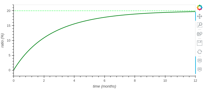
First of all, this is how it looks like when we have an inflationary policy (it can fulfill the common pool up to 20% in one year):

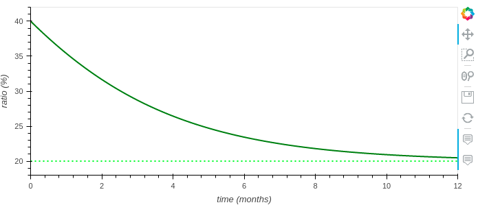
And this is when we enter in deflationary policy (current ratio is higher than target ratio):

If we apply a throttle to the previous charts (max adjustment parameter), we can see how the curve is flat during the first months because we don’t want a very high inflation during any point in time:

And the same happens in deflation if we apply a low enough throttle:

You can play with this model in this jupyter notebook I’ve created (click on Runtime > Run all to play with the sliders).

Some considerations

After playing with the model, I’ve found some problems that I would like to see solved in subsequent versions of the issuance policy, and especially in the one which we will start future gardens.

The current policy doesn’t follow a predictable formula

The current implementation of the formula is iterative. This means that the token supply is adjusted every time a function of the smart contract is called.

This makes difficult to calculate the supply of the token in for example one year from now. The method we can use is to loop 365 times on the adjustment function to find the final common pool balance and token supply. Ideally it should have a formula f(x) where x is the time from now so we can calculate the ratio between the common pool and the token supply.

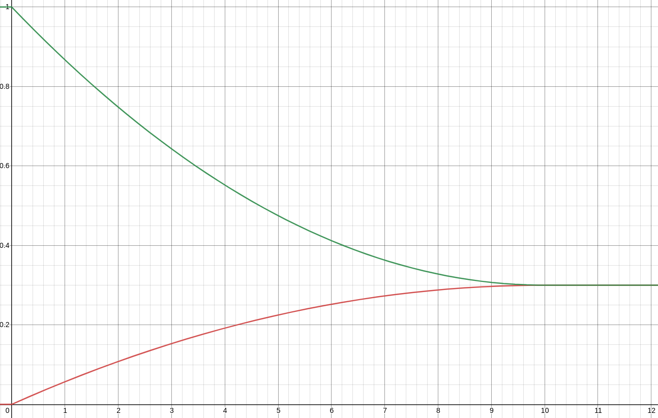
Another problem it has is that due to this iterative behavior, the issuance changes depending on when the function in the smart contract is called. It doesn’t change significantly when it’s called every day, but the divergence is easily observable if we call it once a month (red line):

Parameter name “max adjustment per year” may be misleading

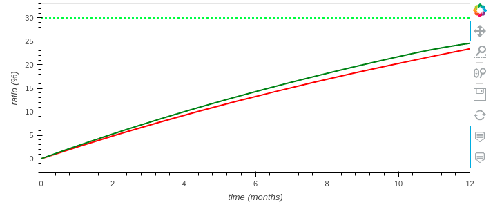
A “max adjustment per year” of 10% doesn’t mean that in one year the total supply won’t increase or decrease more than 10%. For example, setting the initial ratio to 0% and the target ratio is 30% with a “max adjustment per year” of 10%, we see how the total supply is increased by +32.5% in just one year.

We say that it is “max adjustment per year” because the smart contract is requiring a “max adjustment per second” parameter, and we use an annualized input instead. I think it might be misleading so I would simply use the word “throttle” to name this parameter.

The policy acts differently when the ratios are high

Because of the nature of the formula used to calculate the adjustments, it have some odd behaviors when the current or target ratio are high.

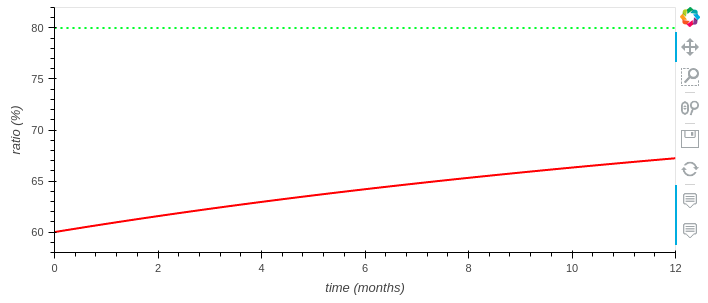
When the target ratio is 80% it takes much more to fill the funding pool than when it is 20% (compare with the first chart):

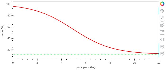
When the current ratio is very high (most of the tokens are in the funding pool), it burns the tokens in a quite strange way:

If you think this is inconsistent, and we could have a nicer issuance policy, I’ve a proposal:

Let’s hack on a better issuance policy!

This is an open call for the Luna Swarm to discuss about the issues with the current dynamic issuance policy and propose a new formula that fits better. Maybe these issues are not concerning enough to change HNY issuance policy, but a Dynamic Issuance v2 with these things solved would be nice before we start the Gardens economies.

[metaverde]

Could you explain how not being able to predict the supply is an issue here?
My understanding is that the dynamic issuance policy is designed to help $HNY maintain a more stable value. In order for the value to remain stable, without being pegged to a stable asset, the supply must be able to fluctuate with the need.
I think that in order for the supply to be predictable the need must be predictable, and we just don’t have that situation.
As an aside, it just occurred to me that we’re effectively working to peg $HNY to our labor.
That’s kind of cool.

If I’m completely misunderstanding how this all works please do let me know.

[sem]

Hello @metaverde, thanks for commenting! I think the post needs some more clarification, I’ll write here what I replied to @willjgriff in discord:

The good thing about having a predictable formula is that you can draw a curve from 0 to target ratio and from 100% to target ratio, and then you know how much time it will cost to go from 10% to 20% for example. If during this time we have an inflow or an outflow, let’s say -5% of the funding pool because a proposal has been funded, then it would be like going back in time, but it would still be predictable how much it would cost to go to target ratio. We can’t predict the behavior of a chaotic system, but we can make their parts simpler to understand.

So the idea is not to change the dynamic issuance policy itself. We won’t be able to predict the supply over time, since it will still be adjusted depending on the funds that there are in the common pool.

The main idea behind this proposal is to be able to have a formula that allows us to understand how common pool will be filled/emptied over time, and to be able to parameterize it.

Today I’ve been working on a formula that could fit properly this propose, and I’m putting here as an example.

Having the parameters:

• t - target ratio
• r - recovery time

We have these formulas to determine the future of the common pool (if no inflows/outflows):

• “Inflationary” formula:
  
• “Deflationary” formula:
  

And this is how it looks like when we configure it with a target ratio of 30% and a recovery time of 10 months:

As you can see, if we start from zero funds in the common pool, the dynamic issuance contract will have minted enough tokens to reach the target ratio of 30%. The contract will burn tokens until the same ratio if we start from a theoretic 100% funds in the funding pool (the whole token supply should not be ever in the funding pool).

If we have for example a 10% of total supply in the common pool, how much it will take to reach 30%? According to the previous graph, it should be less than 8 months (10 months of recovery time - 2 months that it takes to surpass 10%).

If we have a 10% of the funding pool and we receive an inflow of 5% into the funding pool, how much it will take to reach 30%? Probably one month less than if we never received it. The same we when we have an outflow (a conviction voting proposal passes), it is like going back in time, and we need to add more months to pay our common pool “debt” through inflation.

You can play with the target ratio and recovery time parameters in this desmos. It also includes a “current ratio” slider that lets you play with the issuance when you have a ratio in between 0% and 100%.

Take into account that this is only a proof-of-concept, and I’d like to involve more people in the re-design of this important piece of software that might feed the garden economies.

The next I will do is to encode this issuance formula in solidity to see how simple/complex is the required code, stay tuned!

[willjgriff]

The only thing I consider a potential issue here is this: Insights on Dynamic Issuance after modeling it I don’t consider the other aspects particularly important personally.

With that in mind can you explain in a bit more detail how this occurs relating to the formula? Perhaps there’s something small we can change in the current setup to mitigate this without rewriting the whole contract.

[sem]

This is the first chart you are referring to:

To explain it, we have to analyze the Issuance Policy formula:

error = (1 - current_ratio / target_ratio) / seconds_per_year

We see that the adjustment tends to be higher when the target ratio is low, because it’s a number between 0 and 1 which is dividing. When the target ratio is near to 1, we have a very very slow adjustment.

The second chart is this:

This is a behavior that emerges after applying the formula repeatedly, by burning the HNY from the funding pool. When HNY is burnt, the balance of the common pool is reduced, but also does the total token supply. This is why we don’t see much changes when the ratio is close to 100%: we burn a similar amount of both balance and supply, so the ratio is maintained.

I think it is unwilling that a community chooses a high target ratio, so the first problem is not as relevant. And for the second problem, the community could choose to fund many proposals to remove funds from the common pool, so the ratio can go back faster to the target ratio.

The issuance policy v2 is not about solving any big issues of v1 has, it’s more about making it easier to understand, model, and parameterize without odd quirks. We can continue with the current policy as much as we want without any big issue, but since we are releasing the garden economies soon, I think it’s interesting to provide a more modelable formula.