If Honey is Money, understanding the dynamics of the Honey supply is incredibly critical.
Currently we have a simple issuance policy that allows anyone to mint honey to the common pool at a fixed rate per block. This rate can be updated via governance decisions. Currently it is set at approximately 30% per year.
This is relatively high, and reflects the early stage of the community. Just like projects like Bitcoin and Ethereum had high issuance rates early on to help bootstrap a community and economy around their respective assets, the issuance rate for Honey is relatively high currently, and we expect it to be adjusted lower in the future. However, unlike these examples we have not yet codified a process for how the issuance rate is modulated, and instead have relied on governance to come to consensus and make changes as needed.
In line with our general philosophy we want to minimize governance over issuance. One way we could do that would be to replicate a “fixed supply” policy with emissions scheduled years in advance like Bitcoin… however because the goal of the system isn’t just to distribute a finite amount of tokens, but to ensure that the economic engine and incentives of 1Hive participants are aligned we needed to come up with a more sophisticated policy.
- We want to be able to consistently allocate Honey to fund proposals as these proposals are used for development, promotion, and support of new applications that add additional utility to the Honey token.
- We want Honey to remain scarce and increase in value over time.
With this in mind, I with the help of others have been working on a dynamic supply policy that would both issue and burn Honey from the common pool automatically.
We could still allow governance over the hyper parameters of this policy, or choose to remove governance entirely to give people more certainty about the systems behavior. In either case, we would not need to manually adjust the issuance rate, and if we collectively allocate resources productively we should expect to see increases in demand for Honey outpace issuance, either due to Honey being removed from the circulating supply (fee capture), or due to Honey demand increasing as a result of supply sinks (eg staking mechanisms).
Proposed Mechanism
The Dynamic Supply Policy would work similarly to the existing Issuance Policy in that there will be a public function that anyone can call which would adjust the the total supply of Honey.
However, instead of just issuing honey at a fixed rate It will adjust the Total Honey supply in order to target a certain percentage of the total supply in the Common Pool by either issuing new Honey to the Common Pool, or Burning Honey from the Common Pool.
The mechanism makes adjustments to the supply using a proportional control function where the further from the target the system is the greater the magnitude of adjustment are.
error = (1 - current_ratio / target_ratio) / seconds_per_year
This error term tells us how much we should be adjusting the supply to get back to the target ratio. The seconds_per_year constant smooths the adjustments so that even though we can adjust on a per block basis, it would take approximately a year (all else equal) for the system to get back to the target ratio.
To ensure that we can provide a simple and easy to understand upper bound on how quickly the total supply can change over time, we can limit the magnitude of any adjustment by a throttle parameter.
error = (1 - current_ratio / target_ratio) / seconds_per_year

if error < 0:
	adjustment = max(error, -throttle) * supply
else:
  adjustment = min(error, throttle) * supply
In practice the throttle is an artificial limit on the ability for the mechanism to adjust supply, if the throttle kicks in it will take longer for the system to reach the target ratio and may reach an equilibrium that is higher or lower than desired.
From a governance perspective this is useful because we can make it significantly more difficult (or impossible) to adjust the throttle and reserve ratio parameters, while allowing more strategic discretion over the conviction voting parameters that determine the outflow rate from the common pool.
Parameter Choice
In order to adopt the new dynamic supply policy we need to determine what values will be initially used for the target_ratio and throttle .
To help inform our decisions I’ve been working on creating a model of the Honey supply and related economic dynamics of the system. Before getting into those details, conclusions, and proposed values… it’s important to note that all models are imperfect representations of reality but can help to create a better and more robust shared understanding of how we expect the system to behave and make the assumptions we are basing our decisions on more explicit.
Model Overview
I highly encourage anyone interested in the topic to get their hands on the model and play with it, if you have question or aren’t familiar with the tooling, can ask in the Luna channel, or join our weekly working session (each Friday).
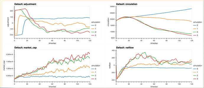
At a high level the model represents the honey protocol as having consistent outflows (conviction proposals), which are used to generate inflows into the common pool based on a production function and market saturation curve.
The dynamic supply policy issues honey to the common pool when below the target ratio, and burns when it is above. Price is modeled as a stochastic processes which gets pulled towards a more deterministic fundamental price that considers inflows and circulating supply to create a valuation.
Based on a model parameter “productivity” we can see that when productivity is too low, the system will not reach a significant percent of market saturation, inflows will not offset outflows, and the supply will increase while the price continues to decline. If productivity is high, the system will reach and stabilize at a high level of market saturation.
This is a relatively simple representation of the economic forces that likely exist within the market, we know that if we pass proposals that are not productive at all, we shouldn’t expect price to increase over the long term, and if we are productive we should expect that to result in an increasing price and market cap for Honey over time.
This productivity parameter is abstract, we may be able to measure productivity of proposals in some way in the future and map that data back into the model, but for now it is just a value that is used to tune the model. Since we don’t know what it actually represents in reality, but we do know that our success is neither guaranteed nor impossible, we can choose an arbitrary productivity value that is neutral and allows us to examine how sensitive success or failure modes are to changes in the throttle and target reserve parameters.
For the target reserve we might have a preference to set the target reserve ratio at the current value to avoid any shocks to the system when we convert over (this is approximately 0.3 presently). We may also want to avoid excessively large values as large values would produce more variability (and discretion using conviction voting) as to the rate funds enter the circulating supply and we may also prefer round numbers given a lack of precise data or guidance.
For the throttle, we are setting an upper bound on the rate at which supply adjustments are made. Likely the most important thing to consider when setting this parameter is what it implies for the maximum issuance rate over time. Currently the issuance rate is ~30% per year, which generally feels quite high if it were to be constant, but may be a reasonable upper bound if we expect it to generally be much lower. A lower value for maximum issuance per year is generally preferred by to members of the community that value long term assurance that inflation will be minimal. On the other hand a value of 0 would imply a fixed supply that cannot adapt to help the system self regulate at all.
With that in mind, I’ve set up the model to do multiple Montecarlo runs (running the same parameters with different random seeds to get a combined data set), across a matrix of parameter choices for target reserve ratio (0.1, 0.2, 0.3, 0.4) and throttle ( 0.004/0.048, 0.008/0.096, 0.016/0.192, 0.025/0.3 — month/year), and with the help of Shawn we have visualizations of the results we can use to understand the impacts of these parameters in the simulations.
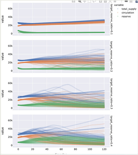
Plotting the total supply, circulation, reserve with trendiness for all the runs, faceted by target reserve ratio we can see clear difference in the choices.
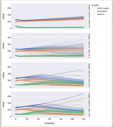
A value of 0.1 has very few instances where totally supply decreases and not a ton of variance between runs. At 0.2 we see more variance with some runs resulting in greater total supply, but also significantly more runs resulting in supply reduction over time, the overall trend line is relatively flat but there there is significant variance between runs. At 0.3 we start to see the trend for total supply become negative, and the rend for circulating supply crossing over. There appears to be a bit less variance across the runs. At 0.4 you have a negative trend as well, but a bit more variance.
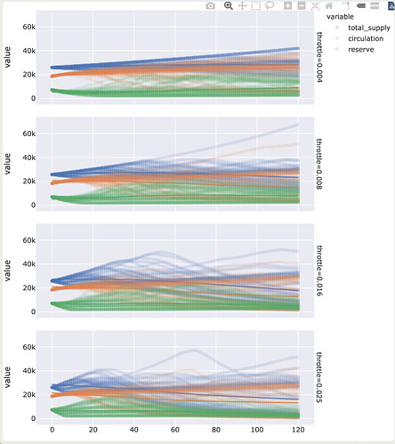
If we look at the same dataset, but we facet by throttle instead of target reserve ratio, we see that the throttle parameter has much less clear trends. Since we generally want to have a lower throttle value to give more certainty about supply adjustments over time, the lack of sensitivity allows us to pick one of the numbers on the lower end.
Let’s say we want to stick to a throttle of 0.008 or or just under 10% per year max issuance, we can run the simulation again and just sweep the target reserve ratio but with a larger number of Monte Carlo runs.
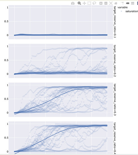
We can also look at the saturation curve, where we see that the there is a pretty significant jump between 0.2 and 0.3, but very little difference between 0.3 and 0.4
We can also plot some of the other variables with their average values across this data set:
And we can see that the 0.3 and 0.4 values for target reserve seem to be fairly similar.
Overall, my impression is that we could go with a value of 0.008 per month which would give us a maximum issuance of less than 10% per year, and a reserve ratio target that is approximately the same as the current state of ~0.3 . I would recommend we start with those values, even though we don’t have a perfect model and can definitely not say that these are the optimal values, they seem to be reasonable values given our analysis.
We could opt to set a strong expectation that the throttle parameter won’t change, as that would give people greater certainty on worst case issuance, with relatively little overall impact on the likelihood of success (at least as far as our model is concerned). But I would encourage us to set the expectation that the target reserve ratio may be changed in the future, if we are able to improve our model, augment it with observed data, and it suggests that a different choice would be better.
We can continue to extend and improve the model, adding and comparing the results of different assumptions, augmenting those assumptions with data that we collect from the system, and use that model to continuously evaluate and inform future governance decisions, parameter adjustments, and policy choices, which is one of the core goals of the Luna Swarm.
Implementation
A solidity implementation of the above dynamic supply policy has been written and can be used to replace our current policy. You can find and review it on https://github.com/1Hive/issuance/blob/master/contracts/Issuance.sol.
This policy has already been incorporated into the test deployment of the 1Hive DAO that includes Celeste integration. Unless there is significant objection to the adoption of this proposal, it likely makes sense to plan to bundle the adoption of the new supply policy with launch of Celeste and adoption of the disputable version of Conviction proposals and decisions.

